Buoyant jet in stagnant ambient

In this example, a horizontal freshwater jet enters an environment of stagnant, salty water. The config.toml file looks like this:

# Characteristics of the pipe and the effluent flow
[pipe]
time = [1970-01-01]
flow = [0.2]
temp = [10]
salt = [0]
diam = [0.5]
depth = [100]
decline = [0]

# Characteristics of the ambient water masses
[ambient]
time = [1970-01-01]
depth = [100]
coflow = [[0]]
crossflow = [[0]]
temp = [[10]]
salt = [[34]]

# Output options
[output]
csv.file = "out.csv"
csv.float_format = "%.6g"
trajectory.step = 5           # Time between trajectory points [s]
trajectory.stop = 30          # Time of final trajectory point [s]
release.start = 1970-01-01    # Time of first release [date]
release.stop = 1970-01-01     # Time of final release [date]
release.step = 3600           # Time between releases [s]

The contents of the output file out.csv is

release_time,t,x,y,z,u,v,w,density,radius,salt,temp,dilution
1970-01-01,0,0,0,100,1.01859,0,0,1000.18,0.25,0,10,1
1970-01-01,5,2.58295,0,99.298,0.321862,0,-0.221547,1018.12,0.712294,23.0643,10,3.11406
1970-01-01,10,3.79528,0,98.001,0.182135,0,-0.284704,1021.79,1.01598,27.7894,10,5.47997
1970-01-01,15,4.52524,0,96.5293,0.117413,0,-0.299837,1023.5,1.29556,29.9897,10,8.48987
1970-01-01,20,5.01937,0,95.0279,0.0834234,0,-0.299357,1024.4,1.56416,31.1482,10,11.943
1970-01-01,25,5.38237,0,93.5428,0.0634415,0,-0.294079,1024.93,1.82395,31.8302,10,15.7213
1970-01-01,30,5.66502,0,92.0884,0.0504749,0,-0.287532,1025.28,2.07582,32.2731,10,19.7595

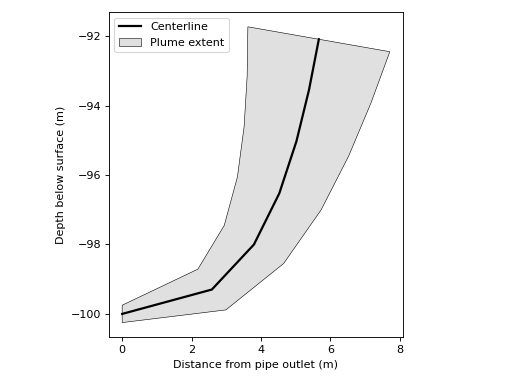
We plot the centerline and plume boundary using matplotlib

import matplotlib.pyplot as plt
import pandas as pd
import numpy as np

df = pd.read_csv("out.csv")

# Compute tangent vector
vel = np.sqrt(df.u.values**2 + df.w.values**2)
tx = df.u.values / vel
tz = df.w.values / vel

# Compute plume boundaries
x1 = df.x.values - df.radius.values * tz
x2 = df.x.values + df.radius.values * tz
z1 = -df.z.values - df.radius.values * tx
z2 = -df.z.values + df.radius.values * tx
x = np.concatenate([x1, np.flip(x2)])
z = np.concatenate([z1, np.flip(z2)])

# Generate figure
plt.plot(df.x.values, -df.z.values, color='k', linewidth=2, label='Centerline')
plt.fill(x, z, edgecolor='k', linewidth=.5, facecolor="#e0e0e0", label='Plume extent')
plt.xlabel('Distance from pipe outlet (m)')
plt.ylabel('Depth below surface (m)')
plt.gca().set_aspect('equal')
plt.legend(loc='upper left')
plt.tight_layout()