Buoyant jet in stratified ambient

In this example, a horizontal freshwater jet is released into a stratified water column. The properties of the pipe outflow and the ambient water masses are specified in external csv files. The config.toml file looks like this:

# Characteristics of the pipe and the effluent flow
[pipe]
csv.file = "pipe.csv"

# Characteristics of the ambient water masses
[ambient]
csv.file = "ambient.csv"

# Output options
[output]
csv.file = "out.csv"
csv.float_format = "%.4f"
trajectory.step = 5           # Time between trajectory points [s]
trajectory.stop = 100          # Time of final trajectory point [s]
release.start = 1970-01-01    # Time of first release [date]
release.stop = 1970-01-01     # Time of final release [date]
release.step = 3600           # Time between releases [s]

Contents of pipe.csv is shown below. For simplicity, this example has constant outflow rates. More lines can be added if the outflow properties are changing with time.

time,       flow, temp, salt, diam, depth, decline
1970-01-01, 0.2,  10,   0,    0.5,  100,   0

Contents of ambient.csv is shown below. More lines can be added to specify further stratification levels, or to specify properties that change with time. Sorting order is not critical, but we recommend sorting by depth, then by time.

time,       depth, coflow, crossflow, temp, salt
1970-01-01, 90,    0,      0,         10,   0
1970-01-01, 110,   0,      0,         10,   34

The contents of the output file out.csv is

release_time,t,x,y,z,u,v,w,density,radius,salt,temp,dilution
1970-01-01,0.0000,0.0000,0.0000,100.0000,1.0186,0.0000,0.0000,1000.1797,0.2500,0.0000,10.0000,1.0000
1970-01-01,5.0000,2.6458,0.0000,99.6487,0.3512,0.0000,-0.1111,1008.7065,0.7056,10.9653,10.0000,2.8805
1970-01-01,10.0000,4.0865,0.0000,98.9911,0.2406,0.0000,-0.1459,1009.9054,0.9754,12.5082,10.0000,4.2051
1970-01-01,15.0000,5.1420,0.0000,98.2385,0.1872,0.0000,-0.1510,1010.2754,1.1961,12.9855,10.0000,5.4036
1970-01-01,20.0000,6.0011,0.0000,97.5142,0.1598,0.0000,-0.1359,1010.3237,1.3866,13.0490,10.0000,6.3343
1970-01-01,25.0000,6.7647,0.0000,96.9035,0.1474,0.0000,-0.1066,1010.2776,1.5515,12.9907,10.0000,6.8792
1970-01-01,30.0000,7.4881,0.0000,96.4653,0.1426,0.0000,-0.0670,1010.2362,1.6955,12.9380,10.0000,7.1132
1970-01-01,35.0000,8.1920,0.0000,96.2422,0.1388,0.0000,-0.0224,1010.1911,1.8212,12.8804,10.0000,7.3224
1970-01-01,40.0000,8.8677,0.0000,96.2394,0.1306,0.0000,0.0204,1010.0855,1.9366,12.7456,10.0000,7.7898
1970-01-01,45.0000,9.4910,0.0000,96.4324,0.1183,0.0000,0.0551,1009.9393,2.0474,12.5591,10.0000,8.5957
1970-01-01,50.0000,10.0507,0.0000,96.7691,0.1058,0.0000,0.0767,1009.8257,2.1566,12.4142,10.0000,9.5474
1970-01-01,55.0000,10.5571,0.0000,97.1753,0.0976,0.0000,0.0832,1009.7885,2.2669,12.3671,10.0000,10.3547
1970-01-01,60.0000,11.0348,0.0000,97.5790,0.0942,0.0000,0.0762,1009.7947,2.3732,12.3753,10.0000,10.7188
1970-01-01,61.4786,11.1739,0.0000,97.6884,0.0940,0.0000,0.0718,1009.7980,2.4034,12.3794,10.0000,10.7337

Observe that integration stopped before the specified end time was reached. This is because the plume at this point has slowed down so much that we have entered the far-field regime, as explained in Algorithm.

We plot the centerline and plume boundary using matplotlib

import matplotlib.pyplot as plt
import pandas as pd
import numpy as np

df = pd.read_csv("out.csv")

# Compute tangent vector
vel = np.sqrt(df.u.values**2 + df.w.values**2)
tx = df.u.values / vel
tz = df.w.values / vel

# Compute plume boundaries
x1 = df.x.values - df.radius.values * tz
x2 = df.x.values + df.radius.values * tz
z1 = -df.z.values - df.radius.values * tx
z2 = -df.z.values + df.radius.values * tx
x = np.concatenate([x1, np.flip(x2)])
z = np.concatenate([z1, np.flip(z2)])

# Generate figure
plt.plot(df.x.values, -df.z.values, color='k', linewidth=2, label='Centerline')
plt.fill(x, z, edgecolor='k', linewidth=.5, facecolor="#e0e0e0", label='Plume extent')
plt.xlabel('Distance from pipe outlet (m)')
plt.ylabel('Depth below surface (m)')
plt.gca().set_aspect('equal')
plt.legend(loc='upper left')
plt.tight_layout()

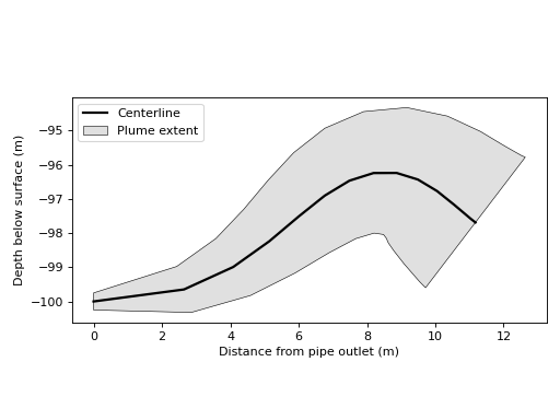
As seen in the figure, the plume is lifted upwards by buoyancy forces. At some point, the plume is diluted so much that its buoyancy is neutral compared to the ambient water masses. It still continues to rise for some time due to its momentum, overshooting the depth level of neutral buoyancy. Eventually, it sinks back into a stable depth level.