Reading ambient data from ROMS
In this example, a horizontal jet of freshwater enters an ocean environment.
The properties of the ambient water masses are taken from the numerical ocean
model ROMS.
The config.toml file looks like this.
# Characteristics of the pipe and the effluent flow
[pipe]
time = [2015-09-07T01:00:00]
flow = [0.2]
dens = [1000]
diam = [0.5]
depth = [20]
decline = [0]

# Characteristics of the ambient water masses
[ambient.roms]
file = "forcing.nc"
latitude = 59.03
longitude = 5.68
azimuth = 45

# Output options
[output]
nc.file = "out.nc"
trajectory.step = 5           # Time between trajectory points [s]
trajectory.stop = 60          # Time of final trajectory point [s]
release.start = 2015-09-07T01:00:00    # Time of first release [date]
release.stop = 2015-09-07T01:00:00     # Time of final release [date]
release.step = 3600           # Time between releases [s]
The input file forcing.nc comes directly from ROMS and contains the
fields u, v, temp and salt. Horizontal coordinates are given by the
variables lat_rho and lon_rho. Vertical coordinates are given by the
variables h, hc, Vtransform and Cs_r. Details about the vertical
coordinate transform is given in the
ROMS documentation.
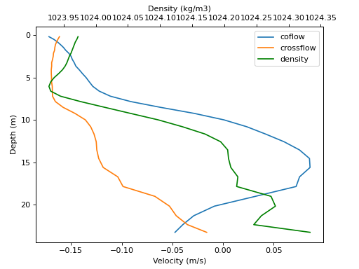
Internally, effluent uses the built-in function load_location to
extract the density and velocity at the given location. Here, we use the same
function for visualization purposes.
import effluent.roms
import matplotlib.pyplot as plt

# Use built-in function to interpolate ROMS data
roms_spec = effluent.roms.load_location(
    file="forcing.nc",
    lat=59.03,
    lon=5.68,
    az=45,
)

# Load roms data
with roms_spec as dset:
    roms = dset.sel(time='2015-09-07 01:00:00')
    depths = roms.depth.values
    dens = roms.dens.values
    u = roms.u.values
    v = roms.v.values

# Prepare plot
ax1 = plt.gcf().add_axes([0.1, 0.1, .8, .8])
ax1.invert_yaxis()
ax2 = ax1.twiny()

# Plot velocity and density
lines = [None] * 3
lines[0] = ax1.plot(u, depths, label='coflow')[0]
lines[1] = ax1.plot(v, depths, label='crossflow')[0]
lines[2] = ax2.plot(dens, depths, label='density', color='g')[0]

# Annotate plot
ax1.set_xlabel('Velocity (m/s)')
ax1.set_ylabel('Depth (m)')
ax2.set_xlabel('Density (kg/m3)')
ax1.legend(handles=lines)
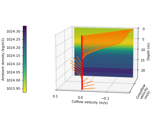
We can visualize the same data in a 3D plot:
from matplotlib.cm import ScalarMappable
from matplotlib.colors import Normalize
import numpy as np

xlims = [u.min(), u.max()]
ylims = [v.min(), v.max()]
zlims = [depths.min(), depths.max()]

# Plot red "velocity pole"
fig = plt.figure()
ax = fig.add_subplot(projection='3d', computed_zorder=False)
ax.invert_zaxis()
ax.plot(xs=[0, 0], ys=[0, 0], zs=zlims,
        color='r', linewidth=4, zorder=100)

# Plot velocity vectors
for d in roms.depth.values:
    u = roms.u.sel(depth=d).values
    v = roms.v.sel(depth=d).values
    ax.plot([0, u], [0, v], [d, d], color='#ff7000', zorder=1)

# Plot ambient density
x, z = np.meshgrid(xlims, depths)
y = ylims[0] * np.ones_like(x)
data_norm = Normalize(dens.min(), dens.max())
data = np.meshgrid(xlims, dens)[1]
rgb = plt.colormaps['viridis_r'](data_norm(data))
ax.plot_surface(x, y, z, zorder=0, facecolors=rgb)

# Annotate plot
ax.set(xticks=[-.1, 0, .1], yticks=[-.1, 0], yticklabels=[])
ax.view_init(elev=10., azim=100)
ax.set_xlabel('Coflow velocity (m/s)')
ax.set_ylabel('Crossflow\nvelocity\n(m/s)')
ax.set_zlabel('Depth (m)')
cmap = fig.colorbar(
    ScalarMappable(norm=data_norm, cmap='viridis_r'),
    shrink=.6,
    ax=ax,
    label='Ambient density (kg/m3)',
    location='left',
)
fig.tight_layout()
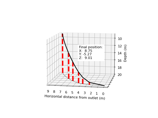
After running effluent, the output is written to the netCDF file out.nc.
We plot the centerline of the plume in a 3D plot
# Load output data
import xarray as xr
import pandas as pd
dset = xr.load_dataset('out.nc')
x = dset.x.isel(release_time=0).values
y = dset.y.isel(release_time=0).values
z = dset.z.isel(release_time=0).values

# Plot stop position
fig = plt.figure()
ax = fig.add_subplot(projection='3d', computed_zorder=False)
ax.invert_zaxis()
for idx in [1, 2, 3, 5, 7, -1]:
    ax.plot(xs=[x[idx]] * 2, ys=[y[idx]] * 2, zs=z[[0, idx]],
            color='r', linestyle='--', linewidth=4, zorder=-1)

# Plot trajectory
ax.plot(x, y, z, color='k', linewidth=2)
ax.plot(x, y, z[0], color='k', linewidth=.5)

# Annotate plot
ax.set(xticks=range(10), yticks=range(-5, 1), yticklabels=[])
ax.view_init(elev=10., azim=100)
ax.set_xlabel('Horizontal distance from outlet (m)')
ax.set_zlabel('Depth (m)')
fig.text(.5, .5,
    'Final position:\n'
    f'X: {x[-1]: .3}\n'
    f'Y: {y[-1]: .3}\n'
    f'Z: {z[-1]: .3}',
    bbox=dict(color='w'),
)